Refactoring
To shorten and modularize the KCSD classes better, I’m moving static functions from KCSD classes to external modules:
- cross_validation.py
- basis_functions.py
- source_distributions.py
- potentials.py
- dist_table_utils.py
- plotting_utils.py
The names are self-explanatory.
The package is more granular now. It makes it much easier to stick to PEP8 rules.
It’s still not fully PEP8, but over ten times closer to that! (flaw count decreased from 500 to 40 by now)
There is some similar code in the KCSD classes so, it could be beneficial to merge them together, however I didn’t find a good way of doing so yet.
Speeding up
Matrices
The matrix operations already look optimized. Nothing special to improve. Contrary to what I supposed in my proposal, there are no sparse matrices in kCSD in general. Some may only appear in the 1D version, which I investigated at that time.
I’m leaving it as it is now. Messing with it will not bring a significant boost.
Integrals
There were serious problems with evaluating double and triple quads, especially when the integrands contained step function.
This is because higher dimensional scipy integrals (nquad, tplquad) don’t handle discontinuities and constant functions well. Triple quads and nquads completely refused to compute potentials with 3D step basis functions.
To overcome this I decided to use other type of integration method - Monte Carlo method.
I came up with Monte Carlo mthod because it handles both gaussian and step function well. Also the calculation time vs precision tradeoff can be manipulated explicitly by specifing the number of sampling points.
Small comparison between Scipy tplquad and Monte Carlo integral:
In [1]: from pykCSD import potentials as pt
In [2]: from pykCSD import basis_functions as bf
In [3]: from pylab import *
In [4]: x = np.array([0.2 * i for i in xrange(20)])
In [5]: R = 1.0
In [6]: h = 0.5
In [7]: pots_tplquad = np.array([pt.b_pot_3d_cont(xp, R, h, 1.0, bf.gauss_rescale_3D) for xp in x])
In [8]: pots_monte = np.array([pt.b_pot_3d_mc(xp, R, h, 1.0, bf.gauss_rescale_3D) for xp in x])
In [9]: plot(x, pots_tplquad)
In [10]: plot(x, pots_monte)
In [11]: show()
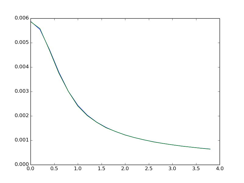
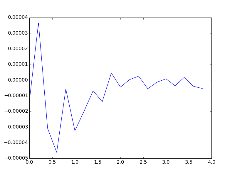
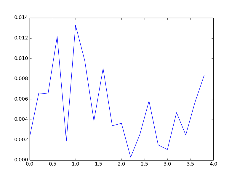
Relative error of Monte Carlo integration method is proportional to inverse square root of the number of samples N, err = and is not dependent on the dimensionality of the integrand.
Using 100000 pts gives average relative error below 1%, which should be low enough for most of reconstructions.
Speed comparison for gausian base and 20 calculations:
%time pots_tplquad = np.array([pt.b_pot_3d_cont(xp, R, h, 1.0, bf.gauss_rescale_3D) for xp in x])
CPU times: user 46.8 s, sys: 0 ns, total: 46.8 s
Wall time: 46.9 s
This takes 46.9 s for SciPy tplquad to complete, now compare to Monte Carlo with 1e5 points:
%time pots_monte = np.array([pt.b_pot_3d_mc(xp, R, h, 1.0, bf.gauss_rescale_3D) for xp in x])
CPU times: user 32 ms, sys: 172 ms, total: 204 ms
Wall time: 19.8 s