TL;DR: - basic version of KCSD3D works, KCSD3D images
During the implementation of the 3D version of kCSD, there were few things to consider:
Distribution of sources in 2D and 3D
Problem: having approx sources we need to distribute them evenly in 3D space.
The approach proposed for two dimensions in kCSD 2D seems a bit unclear to me:
def get_src_params_2D(Lx, Ly, n_src):
	coeff = [Ly, Lx - Ly, -Lx * n_src];

	rts = np.roots(coeff)
	r = [r for r in rts if type(r) is not complex and r > 0]

	nx = r[0]
	ny = n_src/nx

	ds = Lx/(nx-1)

	nx = np.floor(nx) + 1
	ny = np.floor(ny) + 1

	Lx_n = (nx - 1) * ds
	Ly_n = (ny - 1) * ds

	return (nx, ny, Lx_n, Ly_n, ds)
which for enables to distribute sources like this:
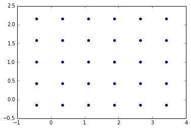
with such parameters:
(nx=6.0, ny=4.0, Lx_n=3.8359071790069814, Ly_n=2.301544307404189, ds=0.76718143580139631)
I have no idea how to extend this into higher dimension.
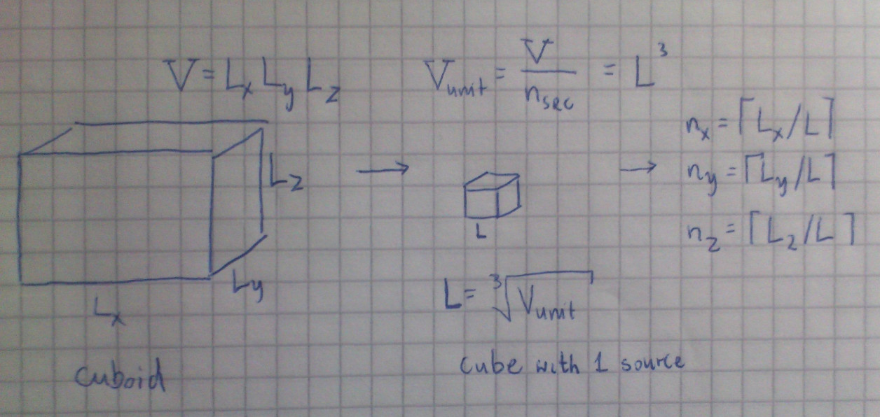
My approach is to divide the area/volume into parts (squares/cubes) and then calculate the side of each square and number of squares for each axis:
def get_src_params_2D_new(Lx, Ly, n_src):
	S = Lx*Ly
	S_unit = float(S)/n_src
	nx = np.ceil(Lx*S_unit**(-1./2))
	ny = np.ceil(Ly*S_unit**(-1./2))

	ds = Lx/nx

	Lx_n = (nx)*ds
	Ly_n = (ny)*ds

	return (nx, ny, Lx_n, Ly_n, ds)
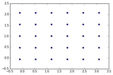
for the same input as in the previous approach it gives slightly different results:
(nx=6.0, ny=4.0, Lx_n=3.2000000000000002, Ly_n=2.1333333333333333, ds=0.53333333333333333)
This scales well from 2D to 3D (and beyond), since it’s based on the conception of (hyper)volume.
Potential
The potential is obviously just:
and may be for example a 3D step function:
which can be imagined as a sphere of uniform density.
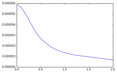
or gaussian function:
which can be imagined as a sphere getting denser and denser near its core.
Calculated at different distances, the function may look like this:
Memory issues
The main matrices used in the kCSD method may become large enough to use whole RAM, let’s investigate them:
- dist_table - O(1), typically 100x1
- this is small and memory-safe
- b_pot_matrix -
- grows fast with number of sources and number of electrodes
- we can suppose this is safe while , (rarely violated)
- b_interp_pot_matrix -
- size grows rapidly with output sampling quality and number of sources
- safe as long as the number of voxels (volume units) (100x100x100) which may not be met for more detailed reconstructions
- b_src_matrix -
- as in b_interp_pot_matrix
- size could be reduced if the basis functions are axis-symmetric, but not in general.
- estimated_pots, estimated_csd -
- size grows rapidly with output sampling quality and number of time records.
- with more than few timeframes, these matrices are impossible to hold in RAM and must be stored on HDD
Plotting
There are few possibilites to visualize 3D data obtained from KCSD.
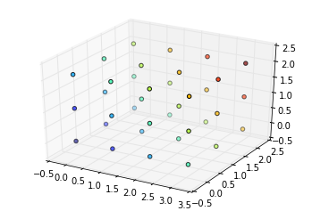
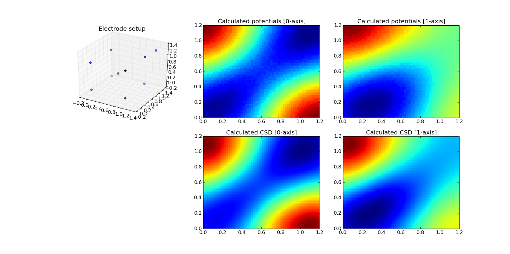
Matplotlib
Matplotlib is designed to visualize 2D data and its 3D features are very limited. We can only visualize electrode positions in 3D as a cloud of points. Potentials and CSD can be presented as slices through chosen axes.
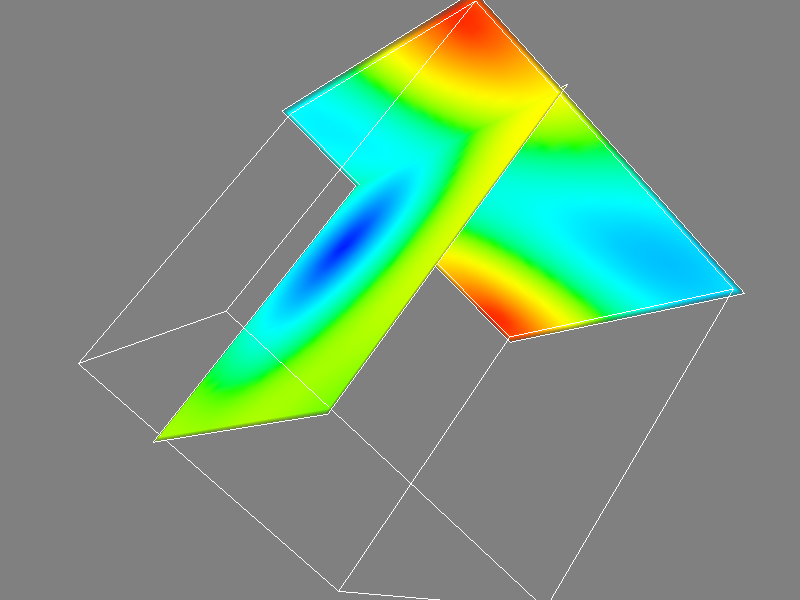
Mayavi
Using mayavi, there are more possibilities:
Plane cuts:
pots = k.estimated_pots
mlab.pipeline.image_plane_widget(mlab.pipeline.scalar_field(pots),
				plane_orientation='x_axes',
				slice_index=10,
				)
mlab.pipeline.image_plane_widget(mlab.pipeline.scalar_field(pots),
				plane_orientation='y_axes',
				slice_index=10,
				)
mlab.outline()
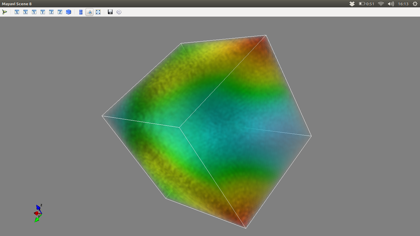
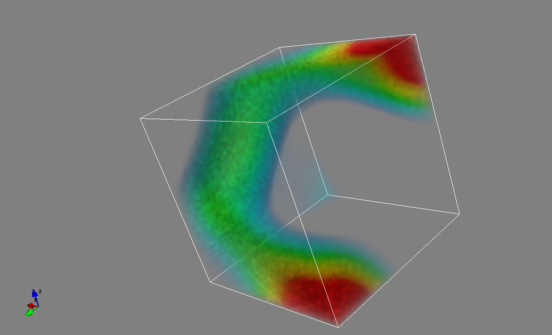
Volumetric plot:
mlab.pipeline.volume(mlab.pipeline.scalar_field(pots))
mlab.outline()
mlab.pipeline.volume(mlab.pipeline.scalar_field(pots),
			vmin=pots.min()+0.2*pots.ptp(),
			vmax=pots.max()-0.2*pots.ptp())
mlab.outline()
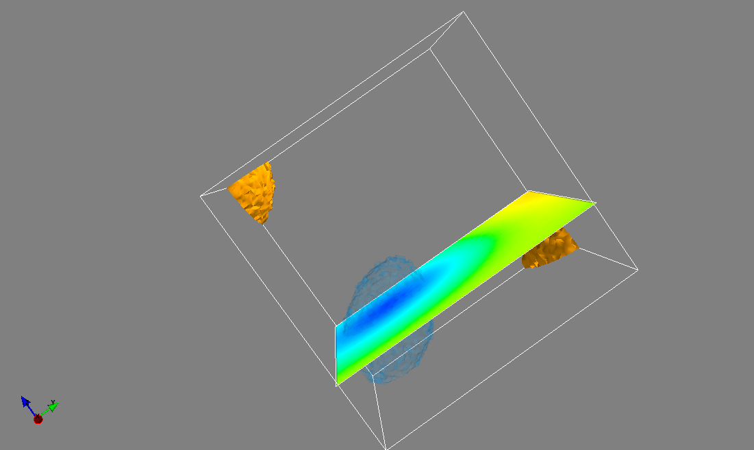
Combined iso-surface and plane cut
s_pots = mlab.pipeline.scalar_field(pots)
mlab.pipeline.iso_surface(s_pots, contours=[pots.min()+0.1*pots.ptp(), ], opacity=0.1)
mlab.pipeline.iso_surface(s_pots, contours=[pots.max()-0.1*pots.ptp(), ],)
mlab.pipeline.image_plane_widget(s_pots,
				plane_orientation='z_axes',
				slice_index=10,
				)
mlab.outline()
PS. to avoid freezes in mayavi.mlab 3D visualizer a proper gui should be used:
%gui wx
External plotter - Paraview
Paraview is a library built for data analysis and visualization. It’s optimized to work with big datasets. Worth a try!
What’s next?
Now that the basic versions of KCSD in 1D, 2D, 3D are implemented, there are few things to manage:
- Refactoring
- improving readability
- reducing code redundancy - each KCSD class is based on the same template. It would be nice to merge them, but only if the code stays readable.
- static functions will be moved to appropriate modules (say: source_templates, source_management, model_potential, cross_validation)
- managing big datasets - some matrices should be read from HDD dynamically and not kept in RAM all the time
- check np.memmap and hdf5 data format
- investigate how much speedup can be achieved
- especially: fix the n-dimensional integrals (numpy warns they don’t converge fast enough), especially if we use step basis.
- investigate if Monte Carlo integration would be useful for triple integrals
- more tests, better documentation
After managing this, the package will be ready to be deployed.